
Zipf's Law
Basic idea
Zipf's Law describes a power law distribution that appears across numerous natural phenomena. The concept is elegantly simple: when you rank items by their frequency or size, the relationship follows a predictable pattern.
Here's how it works: if you arrange items in descending order by their frequency, the Nth item will occur approximately 1/N times as often as the most frequent item. Mathematically, this means:
- The 1st ranked item has frequency X₁
- The 2nd ranked item has frequency X₁/2
- The 3rd ranked item has frequency X₁/3
- The Nth ranked item has frequency X₁/N
This creates a smooth, curved distribution when plotted on a graph, revealing an underlying order in what might initially appear random.
Occurences
Human Language
The most famous application of Zipf's Law is in linguistics. In English, "the" is the most common word, appearing about 7% of the time. "Of" (the second most common) appears roughly half as often at 3.5%. "And" (third) appears about 2.3% of the time. This pattern continues remarkably consistently across languages.
This discovery led linguists to propose Zipf's Law as a litmus test for determining whether a language is artificial or naturally evolved. Real human languages follow this distribution almost universally, while constructed languages often deviate from it.
City Populations
Urban demographics also follow Zipf's Law. In the United States, New York City is the largest with about 8.3 million people. Los Angeles (second largest) has roughly 4 million—close to half. Chicago (third) has about 2.7 million. This pattern holds across countries and time periods.
Passwords
Even in cybersecurity, Zipf's Law emerges. Password frequency distributions follow this pattern, with the most common passwords appearing exponentially more often than less common ones. This has significant implications for security analysis and breach prevention.
Letters
Zipf's law does not occur in letter frequencies since they are not naturally assembled in a dynamical systems but constructed through rigid (human designed) rules.
Deeper Pattern
These occurrences hint at an emergent deeper pattern governing self-organizing natural systems. Zipf's law seems to emerge in complex systems with attractor dynamics.
Relativation: it occurs also for randomly generated words
"In conclusion, Zipf's law is not a deep law in natural language as one might first have thought. It is very much related the particular representation one chooses, i.e., rank as the independent variable." (1) -> Hinting again at a deeper pattern: the observer is part of the observation - the world is inherently subjective and will always look different depending how you look at it.
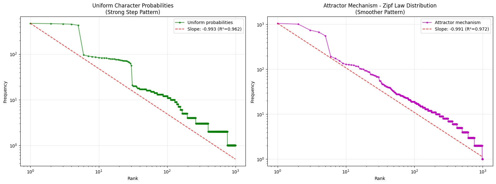
I added an attractor based probability distribution (words that have occurred before are more likely to be sampled, which produces a smoother Zipf curve fit - hinting at attraction effects in natural processes?)
import random
import matplotlib.pyplot as plt
from collections import Counter
import numpy as np
from scipy import stats

attractor_strength = 1.11
ALPHABET = ['a', 'b', 'c', 'd', 'e', '_']  # Example alphabet with underscore as word separator

def calculate_dynamic_attractor_probability(total_words, base_prob=0.16, growth_rate=0.0008, max_prob=0.9):
    """Calculate dynamic attractor probability based on total words generated"""
    # Sigmoid-like growth: starts low, increases with more words, plateaus at max_prob
    dynamic_prob = base_prob + (max_prob - base_prob) * (1 - np.exp(-growth_rate * total_words))
    return min(dynamic_prob, max_prob)

def generate_attractor_text(alphabet, num_chars=100000):
    """Generate random text with dynamic attractor mechanism - probability increases with word count"""
    words = []
    word_counts = {}

    # Start with some initial random words
    text = ''.join(random.choices(alphabet, k=num_chars // 10))
    initial_words = [word for word in text.split('_') if word]

    for word in initial_words:
        words.append(word)
        word_counts[word] = word_counts.get(word, 0) + 1

    # Now generate words with dynamic preferential attachment
    target_length = len(initial_words) * 10

    # Track probability changes for logging
    prob_checkpoints = [len(words) * i // 10 for i in range(1, 11)]

    while len(words) < target_length:
        # Calculate dynamic attractor probability based on total words generated
        current_attractor_prob = calculate_dynamic_attractor_probability(len(words))

        # Log probability at checkpoints
        if len(words) in prob_checkpoints:
            print(f"Words generated: {len(words)}, Attractor probability: {current_attractor_prob:.3f}")

        if word_counts and random.random() < current_attractor_prob:  # Dynamic chance to use existing word
            # Choose existing word with probability proportional to its frequency raised to power
            word_list = list(word_counts.keys())
            weights = [word_counts[word] ** attractor_strength for word in word_list]
            chosen_word = random.choices(word_list, weights=weights, k=1)[0]
            words.append(chosen_word)
            word_counts[chosen_word] += 1
        else:
            # Generate new random word
            word_length = random.randint(1, 5)
            new_word = ''.join(random.choices(alphabet[:-1], k=word_length))
            if new_word:  # Make sure it's not empty
                words.append(new_word)
                word_counts[new_word] = word_counts.get(new_word, 0) + 1

    return words

def generate_li_uniform_text(alphabet, num_chars=100000):
    """Generate random text with uniform character probabilities"""
    text = ''.join(random.choices(alphabet, k=num_chars))
    words = [word for word in text.split('_') if word]
    return words

def calculate_zipf_slope(ranks, frequencies):
    """Calculate Zipf slope using linear regression on log-log scale"""
    log_ranks = np.log10(ranks)
    log_freqs = np.log10(frequencies)

    # Remove infinite values
    valid = np.isfinite(log_ranks) & np.isfinite(log_freqs)
    if np.sum(valid) < 2:
        return None, None

    slope, _, r_value, _, _ = stats.linregress(log_ranks[valid], log_freqs[valid])
    return slope, r_value**2

def plot_attractor_experiment():
    """Generate and plot attractor experiment with uniform comparison"""
    print("Generating attractor mechanism experiment with uniform comparison...")

    # Generate data
    uniform_words = generate_li_uniform_text(ALPHABET)
    attractor_words = generate_attractor_text(ALPHABET)

    print(f"Generated {len(uniform_words)} uniform words and {len(attractor_words)} attractor words")

    # Get frequency distributions
    uniform_counts = Counter(uniform_words).most_common(1000)
    attractor_counts = Counter(attractor_words).most_common(1000)

    # Prepare data for plotting
    uniform_ranks = np.array(range(1, len(uniform_counts) + 1))
    uniform_freqs = np.array([count for _, count in uniform_counts])

    attractor_ranks = np.array(range(1, len(attractor_counts) + 1))
    attractor_freqs = np.array([count for _, count in attractor_counts])

    # Calculate slopes
    uniform_slope, uniform_r2 = calculate_zipf_slope(uniform_ranks, uniform_freqs)
    attractor_slope, attractor_r2 = calculate_zipf_slope(attractor_ranks, attractor_freqs)

    # Create comparison plot
    fig, (ax1, ax2) = plt.subplots(1, 2, figsize=(16, 6))

    # Uniform case
    ax1.loglog(uniform_ranks, uniform_freqs, 'go-', alpha=0.7, markersize=3,
               label='Uniform probabilities')

    if uniform_slope:
        fitted_line = uniform_freqs[0] * (uniform_ranks ** uniform_slope)
        ax1.loglog(uniform_ranks, fitted_line, 'r--', alpha=0.8,
                   label=f'Slope: {uniform_slope:.3f} (R²={uniform_r2:.3f})')

    ax1.set_xlabel('Rank')
    ax1.set_ylabel('Frequency')
    ax1.set_title('Uniform Character Probabilities\n(Strong Step Pattern)')
    ax1.grid(True, alpha=0.3)
    ax1.legend()

    # Attractor case
    ax2.loglog(attractor_ranks, attractor_freqs, 'mo-', alpha=0.7, markersize=3,
               label='Attractor mechanism')

    if attractor_slope:
        fitted_line = attractor_freqs[0] * (attractor_ranks ** attractor_slope)
        ax2.loglog(attractor_ranks, fitted_line, 'r--', alpha=0.8,
                   label=f'Slope: {attractor_slope:.3f} (R²={attractor_r2:.3f})')

    ax2.set_xlabel('Rank')
    ax2.set_ylabel('Frequency')
    ax2.set_title('Attractor Mechanism - Zipf Law Distribution\n(Smoother Pattern)')
    ax2.grid(True, alpha=0.3)
    ax2.legend()

    plt.tight_layout()
    plt.show()

    # Print results
    print(f"\nResults:")
    uniform_slope_str = f"{uniform_slope:.4f}" if uniform_slope is not None else "N/A"
    uniform_r2_str = f"{uniform_r2:.4f}" if uniform_r2 is not None else "N/A"
    attractor_slope_str = f"{attractor_slope:.4f}" if attractor_slope is not None else "N/A"
    attractor_r2_str = f"{attractor_r2:.4f}" if attractor_r2 is not None else "N/A"

    print(f"Uniform case:   slope = {uniform_slope_str}, R² = {uniform_r2_str}")
    print(f"Attractor case: slope = {attractor_slope_str}, R² = {attractor_r2_str}")
    print(f"\nKey finding: The attractor mechanism creates a stronger Zipf-like distribution")
    print(f"compared to uniform probabilities, demonstrating preferential attachment effects.")

# Run the attractor experiment
plot_attractor_experiment()
Closer examination: or does it?
"It is shown that real texts fill the lexical spectrum much more efficiently and regardless of the word length, suggesting that the meaningfulness of Zipf’s law is high." (2) -> Seems Zipf's law is after all not so easily explained...?
Open Questions
Does Zipf's law occur in sentences? -> maybe use semantic sentence clusters (greetings, jokes, etc.) to overcome the uniqueness (frequency 1) challenge of most sentences.
References
- (1) Li, W. (1992). Random Texts Exhibit Zipfs-Law-Like Word Frequency Distribution. IEEE Transactions on Information Theory.
- (2) RAMON FERRER i CANCHO and RICARD V. SOLE. Zipf's Law and Random Texts. Advances in Complex Systems.
- (3) Vsauce. The Zipf Mystery. YouTube.
- (4) Reddit Discussion. Random texts exhibit Zipf's-law-like word frequency distribution. r/voynich.
- (5) Art of the Problem. The Pattern of Intelligence Life. YouTube.
- (6) https://accraze.info/exploring-frequency-distribution-with-chinese-words/